

Introduction 
Copernicus, or COP, is a 2D and 3D GPU image processing framework within Houdini. It allows real-time image manipulation within a 3D space, providing unprecedented flexibility and performance for handling image data. Unlike traditional compositing nodes, Copernicus nodes fully interoperate with SOPs (Surface Operators), enabling seamless integration between 2D and 3D workflows. Copernicus leverages GPU acceleration to provide real-time feedback, making it ideal for interactive workflows. The interoperability with SOP nodes allows users to solve complex problems by choosing the most suitable network type for their tasks. COP nodes can handle both image layers and geometry, giving users the ability to export their work as images or volumes.
Understanding Spaces in Copernicus
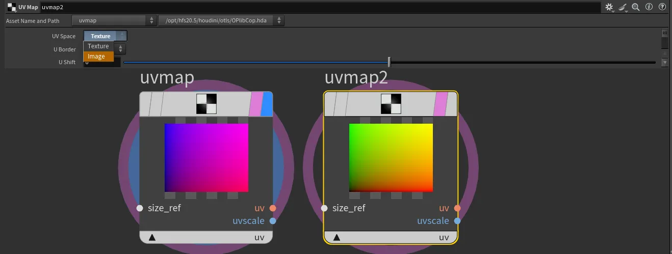
When working with COPs, the default image space ranges from -1 to 1, preserving the pixel aspect ratio. You may also encounter texture space, which ranges from 0 to 1 across the data window and buffer space, useful for mapping textures. Here's a breakdown of the spaces used in Copernicus:
- Buffer Space: Represents the data layout in memory.
- Pixel Space: A canonical pixel-sized area used for precise image manipulation.
- Texture Space: Maps from 0 to 1 across the data window and buffer space, which can result in distorted pixels.
- Image Space: Ranges from -1 to 1 across the display window, preserving the pixel aspect ratio and providing a consistent working area.
- World Space: A 3D location in modeling space. Most users will primarily work within image and texture spaces when using Copernicus nodes, as these spaces are crucial for node operations and visualizations.
Additional Insights
When importing geometry from SOPs and rasterizing it, you might notice that UVs are in the -1 to 1 domain. This is because the positions are being rasterized instead of the actual UVs. The system swaps UV and P (position) for rasterization. If UV mapping is needed, it can be achieved using a UV map, which already has a created correspondence.
Creating a Feedback Loop Solver
Creating a Feedback Loop Solver in COPs In Copernicus context, we can create a "solver" to iterate using a feedback loop.
To set up a solver in COPs, follow these steps:
- Create a Block Node:
Lay down a 'block' node, which will automatically create a Block Start and Block End node pair. These nodes define the start and end points of our feedback loop.
- Add an Invoke Node:
The 'invoke' node is used to control the block. It will repeatedly execute the block of nodes defined between the Block Start and Block End nodes, allowing for iterative processing.
- Specify Input and Output:
You need to manually specify the input and output connections for the Block Start and Block End nodes. Ensure that these connections are consistent and correctly set up to allow data to flow through the loop. Set Inputs and Outputs on the Invoke Node:
Select the Invoke node and click "Set inputs and outputs from selected block." This action will automatically create corresponding input and output connections on the Invoke node that match those on the Block Start and Block End nodes. These connections must match for the feedback loop to function correctly. Adjust Iterations: The number of iterations for the feedback loop can be controlled in the Invoke node settings. This allows you to specify how many times the block should be executed. By default is set to 1, you can set it to $F to behave similarly to a sop solver.
By following these steps, you can create a feedback loop in the COP context, enabling iterative processing and solving.
When creating solvers that utilise 2D vector field, you may be interested in some way of visualising them. Check out this node here
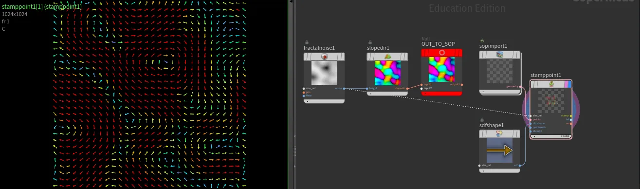
Instancing using geo points
Copernicus also gives us ability to instance(stamp) input image based on geometry points.
stamppoint takes same attributes as a copy sop in its "standard" instancing, but also can utilise sprite specific attributes like spriterot, spritescale, and spriteuv
Passing COPs to Karma
We can pass COP nodes directly to MatrialX shaders with op: path operator ie op:/stage/my_copnet/my_cop_node. This provides great power of the procedural image generation for our renders.
Do not forget to adjust your dicing setting when working with displacements smaller than your polygon size!
Passing COPs to SOPs
Simiraly as passing COPs to Karma, we can pass COPs data to SOPs, using op: operator, same way as we used to in "old COP" network. v@Cd = colormap("op:"+chs("cop"), @uv);. This of course will work with any node that is expecting image file path.
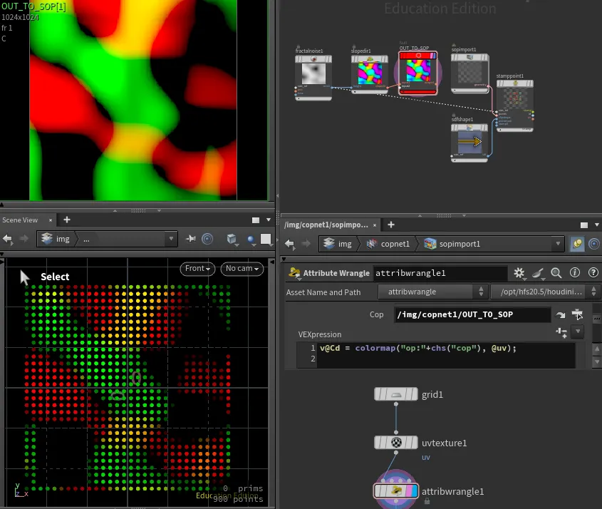
We can use this technique as an alternative for creating things like 2D vector visualizer, without the need for vex or opencl.
Introduction
With Copernicus, a refreshed COPnet in Houdini 20.5, OpenCL knowledge is becoming more and more useful for everyday artists.
Getting Started
When we create a new OpenCL node inside a COP network, we are presented with pre-defined helper code and some setup options under the Signature tab:
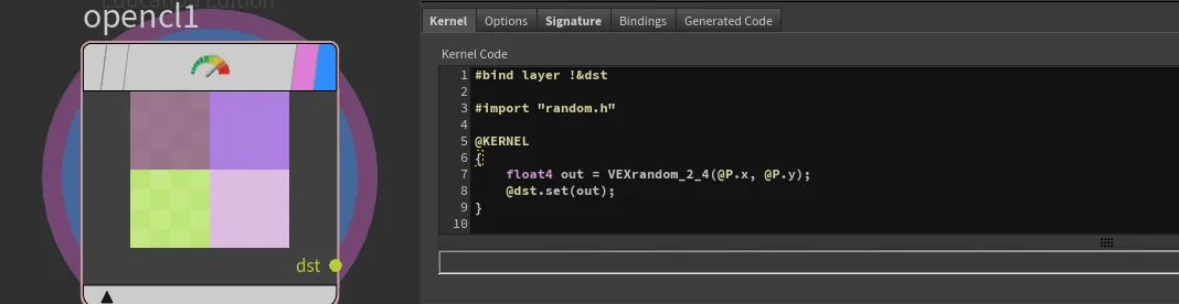
#bind layer src? val=0
#bind layer !&dst

@KERNEL
{
    @dst.set(@src);
}
Let's start with the Signature tab first.
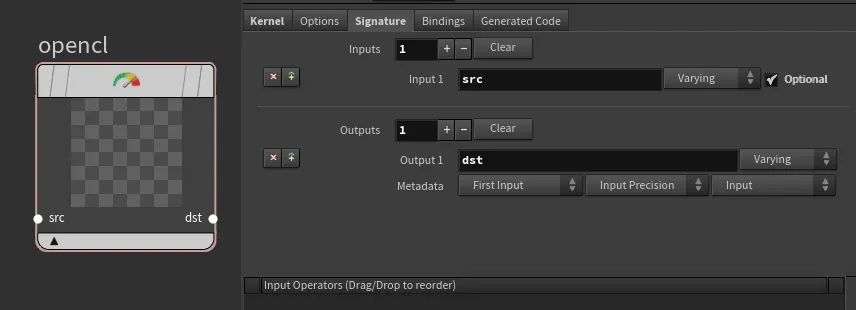
The first lines with #bind are here to specify the input/output for the code.
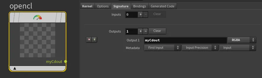
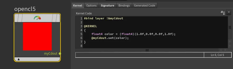
#bind layer src? val=0This tells us that we are expecting a src layer which is optional (?) and its default value is 0 unless specified by the input. Since we have removed the src input under the Signature tab, we should also remove it from the code.#bind layer !&dst: This tells us that we are expecting a dst layer which is required (!) and it is bound as an output buffer or a writable layer (&`). Since we have renamed the output from dst to myCdout, let's reflect that as well.
The @KERNEL block is the main function where our logic goes:
@dst.set(@src); - This means that the values from the src layer are copied to the dst layer. You can read about other attribute binding methods here
Since we have renamed dst to myCdout and removed src, we should update our code accordingly:
#bind layer !&myCdout

@KERNEL
{
    @myCdout.set();
}
At this moment, our code will still fail because we are not binding anything to the output myCdout yet. So let's define some output. We can start with a simple color red (1.0, 0.0, 0.0, 1.0).
Unlike VEX, we cannot specify a new attribute type as vector. OpenCL uses a slightly different type notation OpenCL types.
The equivalent of vector in OpenCL is float3, but in our case, we want to output RGBA, so we will use float4 to include the fourth (alpha) component.
In VEX, we would write:
vector4 color = set(1.0, 0.0, 0.0, 1.0);
In OpenCL, the equivalent would be:
float4 color = (float4)(1.0f,0.0f,0.0f,1.0f);
Our last step is to pass the newly created color attribute to the myCdout output binding:
#bind layer !&myCdout

@KERNEL
{
    float4 color = (float4)(1.0f,0.0f,0.0f,1.0f);
    @myCdout.set(color);
}
And done! We have created a red color in OpenCL!
Adding Spare parameters
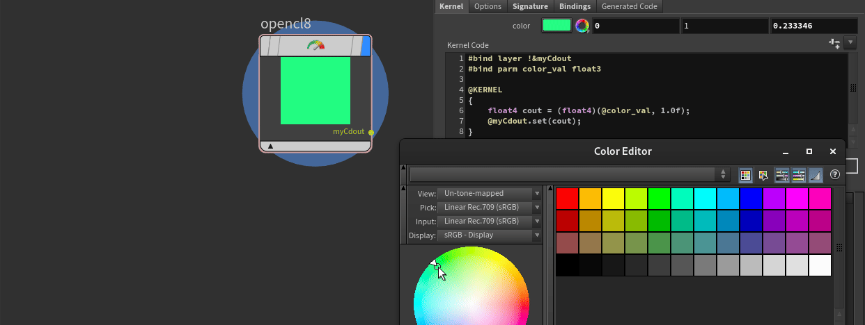
Now, let's add one last feature: the ability for the user to specify their own color within the UI.
Similarly to VEX bindings, we have some automated spare parameter creation features. In VEX, if we would write chf("my_parm"), the OpenCL equivalent would be #bind parm my_parm float. While in VEX we can write bindings anywhere within our code, in OpenCL they must be provided outside the @KERNEL{} function, preferably at the very top of your code block, along with other bindings.
In the Kernel code tab, let's add:
#bind parm color_val float3Now, just like with VEX bindings, you can click the top right corner button to create a spare parameter.
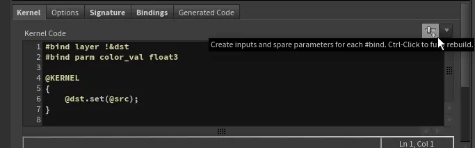
This magical button performs two steps for us:
- It adds a new spare parameter under the Bindings tab, setting up a matching name to our #bind directive with the corresponding data type.
- It adds a UI spare parameter of the selected type and links it as a relative reference.
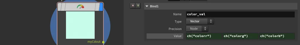
And that's it! Now you have linked a spare parameter to your code. To reference it within your code, all you have to do is use the @ sign, which, unlike in VEX where it imports a global attribute, in OpenCL it refers to a binding name. Therefore, in our case, it is just @color_val.
However, to make this code usable, there is one last issue to address. We have specified a spare parameter of a vector (float3) type, while our default OpenCL output is expecting an RGBA (float4) type. We can utilize OpenCL's swizzle operator to provide the last, missing fourth element for the Alpha:
float4 color = (float4)(@color_val, 1.0f);Our updated kernel code looks like this:
#bind layer !&myCdout
#bind parm color_val float3

@KERNEL
{
    float4 color = (float4)(@color_val, 1.0f);
    @myCdout.set(color);
}
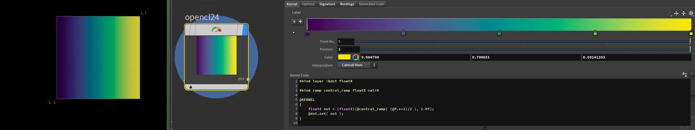
Bind ramp to control Opencl values
If we want to use ramp spare parameter to control values within opencl, first lets add ramp inside bindings tab. I am going to name mine 'control_ramp'
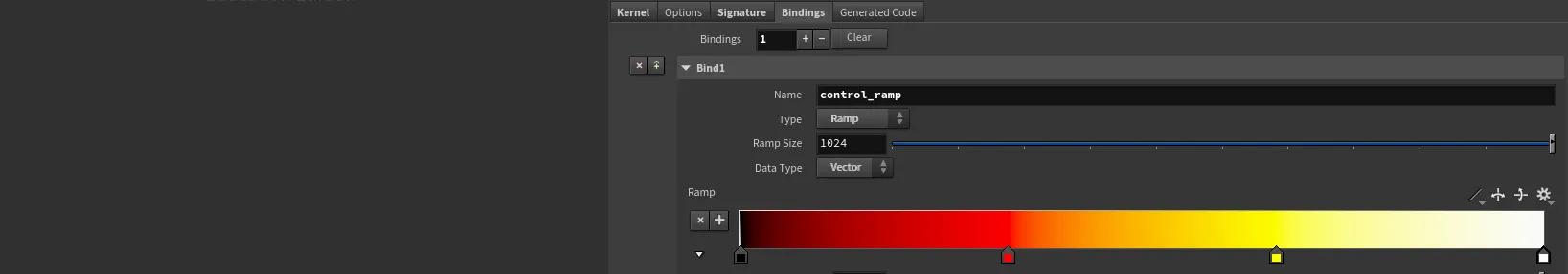
@P. We have to remember that in COPs pixel position is bound between -1 and 1, therefore we will have to normalize values first
(@P.x+1)/2Now, having values between 0-1, if we want to sample ramp, first we need to declare new bind as a ramp
#bind ramp control_ramp float3 val=0next, we can use bound ramp name @control_ramp like a function that accepts sample position
@control_ramp( (@P.x+1)/2 )And that's it! we now, can remap image X by ramp spare parameter!
#bind layer !&dst float4

#bind ramp control_ramp float3 val=0

@KERNEL
{
    float4 out = (float4)(@control_ramp( (@P.x+1)/2 ), 1.0f);
    @dst.set( out );
}
Swirly patterns
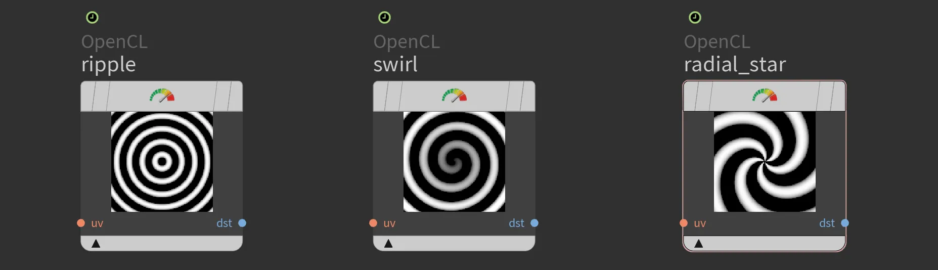
Radial ripple
To achieve the radial ripple effect, we calculate the sine of the distance from the centroid. The default domain is from -1 to 1. To add artistic control, we can introduce period and phase parameters. These can be promoted and linked to expressions like $T for animation.
#bind layer uv? float2
#bind layer !&dst

#bind parm amplitude float
#bind parm period float
#bind parm phaze float

@KERNEL
{
    float2 uv = @uv;
    if(!@uv.bound){
        uv = @P;
    }

    float4 C = @amplitude * sin(length(uv)/@period+@phaze);
    @dst.set(C);
}
Swirl
The swirl pattern is created by calculating the radius and angle for each point, then modifying the angle based on the radius. This creates a spiral effect, with the swirl strength controlled by the period and phase parameters.
#bind layer uv? float2
#bind layer !&dst

#bind parm amplitude float
#bind parm phase float
#bind parm period float

@KERNEL
{
    float2 uv = @uv;
    if(!@uv.bound){
        uv = @P;
    }

    // Calculate the radius and angle
    float radius = length(@P);
    float angle = atan2(uv.y, uv.x);

    // Create a swirl effect by modifying the angle based on the radius
    angle += @phase + @period * radius;

    // Convert back to Cartesian coordinates
    float out = (radius * cos(angle)) * @amplitude;

    @dst.set(out);
}Radial star
The radial star pattern uses sine waves based on both the distance from the center and the angle around the center. By varying these parameters, we create a star-like pattern that can animate over time.
#bind layer uv? float2
#bind layer !&dst

#bind parm time float

@KERNEL
{
    float2 uv = @uv;
    if(!@uv.bound){
        uv = @P;
    }

    float distance = length(@P);
    float angle = atan2(uv.y, uv.x);

    float star = sin(10.0 * distance - 5.0 * angle + @time);

    @dst.set(star);
}You can grab file with those examples,
Wavey patterns
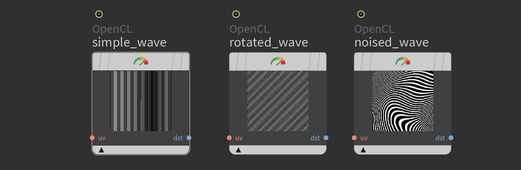
Simple wave
#bind layer uv? float2
#bind layer !&dst

#bind parm scale float val=200
#bind parm phase float val=0

@KERNEL
{
    float2 uv = @uv;
    if(!@uv.bound){
        uv = @P;
    }

    // Create wave pattern
    float wave = sin(uv.x * @scale + @phase);

    @dst.set(wave);
}Rotated wave
Vanilla OpenCL does not have many mathematical functions built in. SideFX team have build helping functions for matrix operations but for this, simple rotation we could just utilise simple sin() and cos() functions to apply rotations.
#bind layer uv? float2
#bind layer !&dst float

#bind parm scale float val=200
#bind parm phase float val=0
#bind parm rotation float val=45

// Function to create a wave pattern based on UV coordinates
float wave(float2 uv, float scale, float phase, float rotation) {
    // Convert rotation to radians
    float rad = radians(rotation);

    // Calculate the rotated UVs
    float u = uv.x * cos(rad) - uv.y * sin(rad);
    float v = uv.x * sin(rad) + uv.y * cos(rad);

    // Create the wave pattern
    float wave = sin(u * scale + phase);

    return wave;
}

@KERNEL
{
    float2 uv = @uv;
    if (!@uv.bound) {
        uv = @P;
    }

    float result = wave(uv, @scale, @phase, @rotation);

    @dst.set(result);
}Noised wave
To make our wave more interesting, we could apply some noise. But, as I have mentioned above, vanilla opencl is quite bare and it does not provide any build-in noises like a common gradient noise Perlin Noise. Implementing it on our own might be overwhelmin, therefore we could piggyback on SideFX pre-built functions from mtlx_noise_internal.h like
mx_perlin_noise_float_2(float2 p, int2 per)
mx_perlin_noise_float_3(float3 p, int3 per)
mx_perlin_noise_float3_2(float2 p, int2 per)
mx_perlin_noise_float3_3(float3 p, int3 per)#bind layer uv? float2
#bind layer !&dst float
#bind parm scale float val=200
#bind parm phase float val=0
#bind parm rotation float val=45
#bind parm distortion float val=0.6
#import "mtlx_noise_internal.h"
// Function to create a wave pattern with distortion
float wave(float2 uv, float scale, float phase, float rotation, float distortion) {
// Convert rotation to radians
float rad = radians(rotation);
// Calculate the rotated UVs
float u = uv.x * cos(rad) - uv.y * sin(rad);
float v = uv.x * sin(rad) + uv.y * cos(rad);
// Apply noise for distortion using Perlin noise
float noiseValue = mx_perlin_noise_float_2((float2)(u, v), (int2)(0, 0)) * distortion;
// Create the wave pattern with distortion
float wave = sin((u + noiseValue) * scale + phase);
return wave;
}
@KERNEL
{
float2 uv = @uv;
if (!@uv.bound) {
// Convert @P from range [-1, 1] to [0, 1]
uv = (@P + 1.0f) * 0.5f;
}
float result = wave(uv, @scale, @phase, @rotation, @distortion);
@dst.set(result);
}You can grab file with those examples,
Noise Functions in OpenCL
Vanilla OpenCL does not provide any build-in noise functions but thanks to Sony Pictures Imageworks and the SideFX team, we have a modified version of osl noise library avaiable for import.
#import "mtlx_noise_internal.h"Within the file we can find variety of functions for us to use, like:
Perlin Gradient Noise Functions
float mx_perlin_noise_float_2(float2 p, int2 per)
float mx_perlin_noise_float_3(float3 p, int3 per)
float3 mx_perlin_noise_float3_2(float2 p, int2 per)
float3 mx_perlin_noise_float3_3(float3 p, int3 per)Description: These functions generate Perlin gradient noise for a given point p. The per parameter specifies the periodicity along each axis, allowing for tileable noise. The functions return either a single float or a float3 result, depending on the input dimensions and the specific function used.
Worley Noise Functions
float mx_worley_noise_float_2(float2 p, float jitter, int metric, int2 per)
float mx_worley_noise_float_3(float3 p, float jitter, int metric, int3 per)
float2 mx_worley_noise_float2_2(float2 p, float jitter, int metric, int2 per)
float2 mx_worley_noise_float2_3(float3 p, float jitter, int metric, int3 per)
float3 mx_worley_noise_float3_2(float2 p, float jitter, int metric, int2 per)
float3 mx_worley_noise_float3_3(float3 p, float jitter, int metric, int3 per)Description: These functions compute Worley noise for a given point p with an added jitter and a specified distance metric (Euclidean, Manhattan, or Chebyshev). The per parameter sets the periodicity for tiling. The functions return either the closest squared distance(s) or vectors depending on the input dimensions and the specific function used.
Utility Hash Functions
uint mx_hash_int1p(int x, int px)
uint mx_hash_int2p(int x, int y, int px, int py)
uint mx_hash_int3p(int x, int y, int z, int px, int py, int pz)
uint mx_hash_int4p(int x, int y, int z, int xx, int px, int py, int pz, int pxx)Description: These functions generate a hash value for integer coordinates with optional periodic wrapping defined by px, py, pz, and pxx.
Noise Conversion Functions
float mx_cell_noise_float_1(float p, int per)
float mx_cell_noise_float_2(float2 p, int2 per)
float mx_cell_noise_float_3(float3 p, int3 per)
float mx_cell_noise_float_4(float4 p, int4 per)
float3 mx_cell_noise_float3_1(float p, int per)
float3 mx_cell_noise_float3_2(float2 p, int2 per)
float3 mx_cell_noise_float3_3(float3 p, int3 per)
float3 mx_cell_noise_float3_4(float4 p, int4 per)Description:
These functions generate cellular noise for given input dimensions p and periodicity per. They return either a single float or a float3 value representing the noise value.
Interpolation Functions
Bilinear and Trilinear Interpolation
float mx_bilerp1(float v0, float v1, float v2, float v3, float s, float t)
float3 mx_bilerp3(float3 v0, float3 v1, float3 v2, float3 v3, float s, float t)
float mx_trilerp1(float v0, float v1, float v2, float v3, float v4, float v5, float v6, float v7, float s, float t, float r)
float3 mx_trilerp3(float3 v0, float3 v1, float3 v2, float3 v3, float3 v4, float3 v5, float3 v6, float3 v7, float s, float t, float r)Description: These functions perform bilinear and trilinear interpolation on float and float3 values, respectively, using the given interpolation parameters s, t, and r.
Gradient Functions
float mx_gradient_float1_2(uint hash, float x, float y)
float mx_gradient_float1_3(uint hash, float x, float y, float z)
float3 mx_gradient_float3_2(uint3 hash, float x, float y)
float3 mx_gradient_float3_3(uint3 hash, float x, float y, float z)Description: These functions compute gradient values based on the given hash and coordinates. They are used internally in noise functions to determine the contribution of each grid point.
Fractal Noise Functions
float mx_fractal_noise_float(float3 p, int octaves, float lacunarity, float diminish, int3 per)
float3 mx_fractal_noise_float3(float3 p, int octaves, float lacunarity, float diminish, int3 per)
float2 mx_fractal_noise_float2(float3 p, int octaves, float lacunarity, float diminish, int3 per)
float4 mx_fractal_noise_float4(float3 p, int octaves, float lacunarity, float diminish, int3 per)Description: These functions generate fractal noise by combining multiple octaves of Perlin noise. The octaves, lacunarity, diminish, and per parameters control the frequency, amplitude, and periodicity of the noise.
Miscellaneous Utility Functions
uint mx_rotl32(uint x, int k)
void mx_bjmix(uint* a, uint* b, uint* c)
uint mx_bjfinal(uint a, uint b, uint c)
float mx_bits_to_01(uint bits)
float mx_fade(float t)Description: These utility functions perform various tasks such as bitwise rotation, mixing and finalizing hash values, converting bits to a float in the range [0, 1], and computing the fade curve for interpolation.
Example of mx_fade() function:
#bind layer uv? float2
#bind layer !&dst float

#include "mtlx_noise_internal.h"

@KERNEL
{
    float2 uv = @uv;

    if(!@uv.bound){
        // Convert @P from range [-1, 1] to [0, 1]
        uv = (@P + 1.0f) * 0.5f;
    }

    // Draw a thin line between (0, 0) and (1, 1)
    float line_thickness = 0.01f;
    float distance_to_line = fabs(uv.x - uv.y);

    // Apply mx_fade to both UV coordinates for a smoother transition
    float faded_u = mx_fade(uv.x);
    float faded_v = mx_fade(uv.y);

    // Combine the faded values to create a result
    float distance_to_faded_line = fabs(faded_u - faded_v);
    float faded_line_value = distance_to_faded_line < line_thickness ? 1.0f : 0.0f;

    // Set the result to the destination layer
    @dst.set(faded_line_value);
}

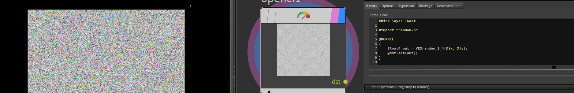
Random numbers in OpenCL
Similarly to Noise functions, we also have random number generators within the random.h file.
You can import it same way as our noise patterns
#import "random.h"static float VEXrandom_1_1(float x)
static float2 VEXrandom_1_2(float x)
static float3 VEXrandom_1_3(float x)
static float4 VEXrandom_1_4(float x)
static float VEXrandom_2_1(float x, float y)
static float2 VEXrandom_2_2(float x, float y)
static float3 VEXrandom_2_3(float x, float y)
static float4 VEXrandom_2_4(float x, float y)
static float VEXrandom_3_1(float x, float y, float z)
static float2 VEXrandom_3_2(float x, float y, float z)
static float3 VEXrandom_3_3(float x, float y, float z)
static float4 VEXrandom_3_4(float x, float y, float z)
static float VEXrandom_4_1(float x, float y, float z, float w)
static float2 VEXrandom_4_2(float x, float y, float z, float w)
static float3 VEXrandom_4_3(float x, float y, float z, float w)
static float4 VEXrandom_4_4(float x, float y, float z, float w)Description:
This set of functions mimics VEX random() function. Depending on your scenario, you may want to input float-float4 and output float-float4
side note:
When using VEXrandom function, you could be thinking that it would create a white noise when passing lets say @P. But actually, as its vex equivalent, this function converts the floating point argument to an integer seed.
@P,@uv or use something like @iy @iy (buffer integer index)
Fabric patterns
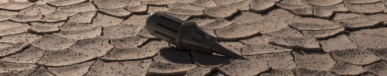
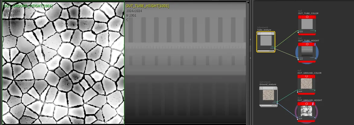
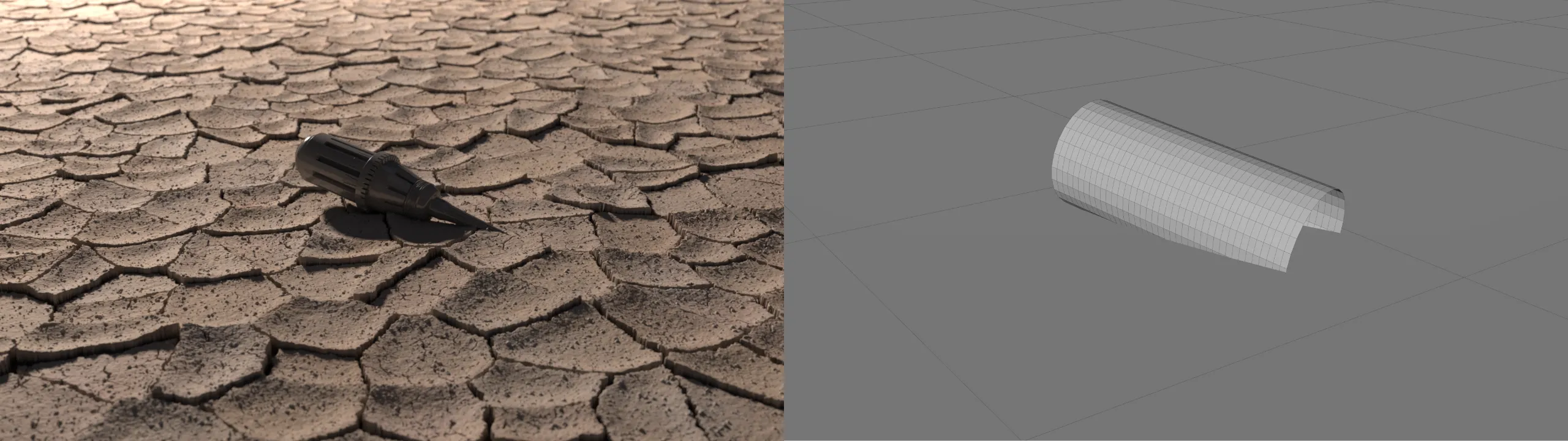
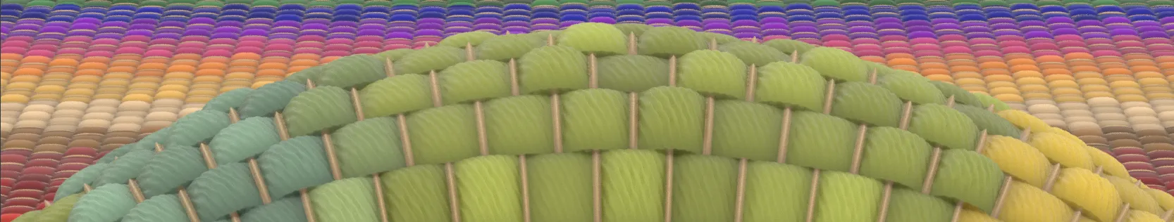
With the refreshed COP network we can do more than just 2D fancy patterns, we can actually utilize them as a procedural textures!. One example to consider is procedural fabric. Due to the complexity of detail, artists quite often 'bake' 3D pattern into texture, which then is applied on a 3D model. Here is just an example where we could utilize power of COP network and fully generate complex pattern which then could be linked into Karma/MaterialX shaders.
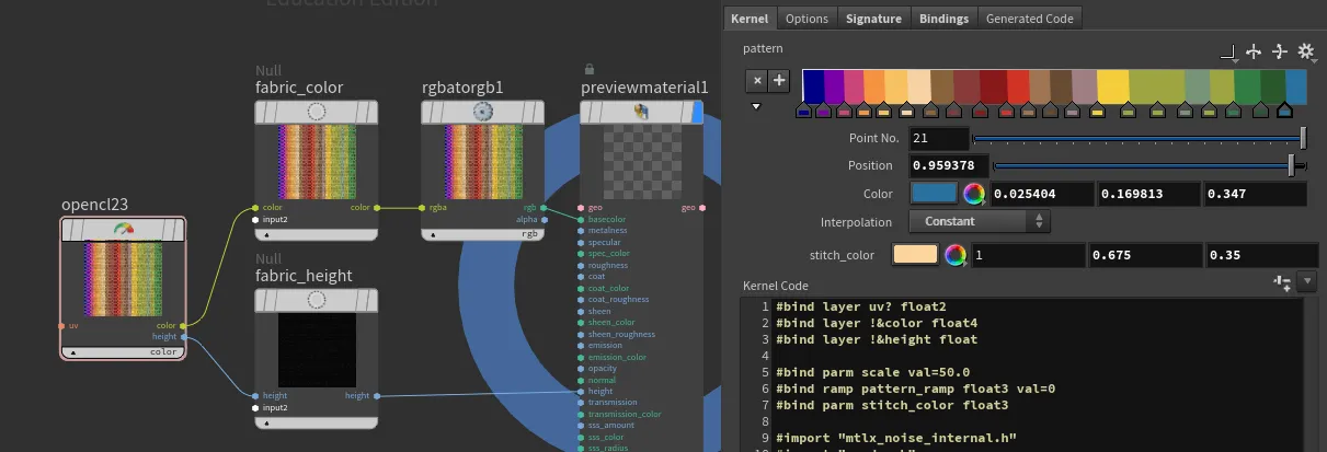
#bind layer uv? float2
#bind layer !&color float4
#bind layer !&height float

#bind parm scale val=50.0
#bind ramp pattern_ramp float3 val=0
#bind parm stitch_color float3

#import "mtlx_noise_internal.h"
#import "random.h"

float pingpong(float x, float scale) {
    x = x / scale;
    return scale * (1.0f - fabs(fmod(x, 2.0f) - 1.0f));
}

float snap(float x, float increment) {
    return increment * floor(x / increment);
}

float s_curve(float x, float k, float x0) {
    return 1.0f / (1.0f + exp(-k * (x - x0)));
}

float lighten(float a, float b, float factor) {
    return mix(a, max(a, b), factor);
}

float2 rand2(float2 uv, float factor) {
    float2 randValues = VEXrand_2_2(uv.x, uv.y);
    return mix((float2)(1.0f, 1.0f), randValues, factor);
}

float wave(float2 uv, float scale, float phase, float rotation, float distortion, float roughness) {
    float rad = -radians(rotation);
    float u = uv.x * cos(rad) - uv.y * sin(rad);
    float v = uv.x * sin(rad) + uv.y * cos(rad);
    float noiseValue = mx_perlin_noise_float_2((float2)(u, v)*(roughness*10), (int2)(0, 0)) * distortion*.01;
    float wave = (sin((u + noiseValue) * 20 * scale + phase)+1)/2;
    return wave;
}

float4 adjust_value(float4 color, float value_adjustment) {
    float value = fmax(color.r, fmax(color.g, color.b));
    float new_value = clamp(value + value_adjustment, 0.0f, 1.0f);
    float scale = (value > 0.0f) ? (new_value / value) : 0.0f;
    float3 adjusted_rgb = color.rgb * scale;
    adjusted_rgb = clamp(adjusted_rgb, 0.0f, 1.0f);
    return (float4)(adjusted_rgb, color.a);
}

float2 perlin(float2 uv, float turbulence, float2 offset, float phase, float amplitude, float roughness) {
    uv += offset;
    float noiseValue = mx_perlin_noise_float_2(uv * (roughness * 10) + phase, (int2)(0, 0)) * amplitude;
    float turbulenceValue = noiseValue * turbulence;
    uv += (float2)(turbulenceValue, turbulenceValue);
    return uv;
}

@KERNEL
{
    // Bind the UV coordinates
    float2 uv = @uv;
    if(!@uv.bound){
        // Convert @P from range [-1, 1] to [0, 1]
        uv = (@P + 1.0f) * 0.5f;
    }
    uv = mix(perlin(@uv, 2, (float2)(0.1f, 0.1f), .5, .05, .6), uv, .95);
    uv *= @scale;
    float2 dscale = (float2)(3.0f, 1.0f);
    uv *= dscale;

    // Calculate xrows and xstripe
    float xrows = fmod(uv.y, 2) > 1 ? 1 : 0;
    float xstripe = pingpong(uv.y, 0.5) * 2;
    float ystripe = pingpong(xrows + uv.x, 1);
    float stitch = 1 - (fmin(0.1f, ystripe) / 0.1f);

    // Calculate patches and texture color
    float2 patches = ((float2)(snap(xrows + uv.x, 2), floor(uv.y)) / dscale) / @scale;
    float4 tex = (float4)(@pattern_ramp(patches.x), 1.0f);
    float4 stitch_color = (float4)(@stitch_color, 1.0f);

    // Mix texture color with stitch color based on stitch value
    float4 cout = mix(tex, stitch_color, stitch > 0 ? 1 : 0);

    // Compute the wave pattern with distortion
    // Define parameters
    float scale = 1.9;
    float phase = 1;
    float rotation = 45.0f; // Rotation in degrees
    float distortion = 4; // Distortion factor
    float roughness = .5; // Distortion factor
    float outwave = wave(uv, scale, rand2(patches,1).y*10, rotation, distortion, roughness)*0.1;

    // height
    float k = 6.0f; // Steepness of the S-curve
    float x0 = 0.2f; // Midpoint of the S-curve
    float hx = s_curve(ystripe, k, x0);
    float hy = s_curve(xstripe, k, 0.1);
    hx*=hy;
    hx *= 1-outwave;
    float stitch_shape = s_curve(stitch*.6, 4, 0.2)*s_curve(xstripe, k, 0.2);
    hx = lighten(hx* rand2(patches,.6).x , stitch_shape, .6);

    cout = adjust_value(cout, 1-rand2(patches+34,0.25).x);
    cout *= pow((float4)(hx, hx, hx, 1), .5);
    hx *= (0.3 / @scale);

    @color.set(cout);
    @height.set(hx);
}
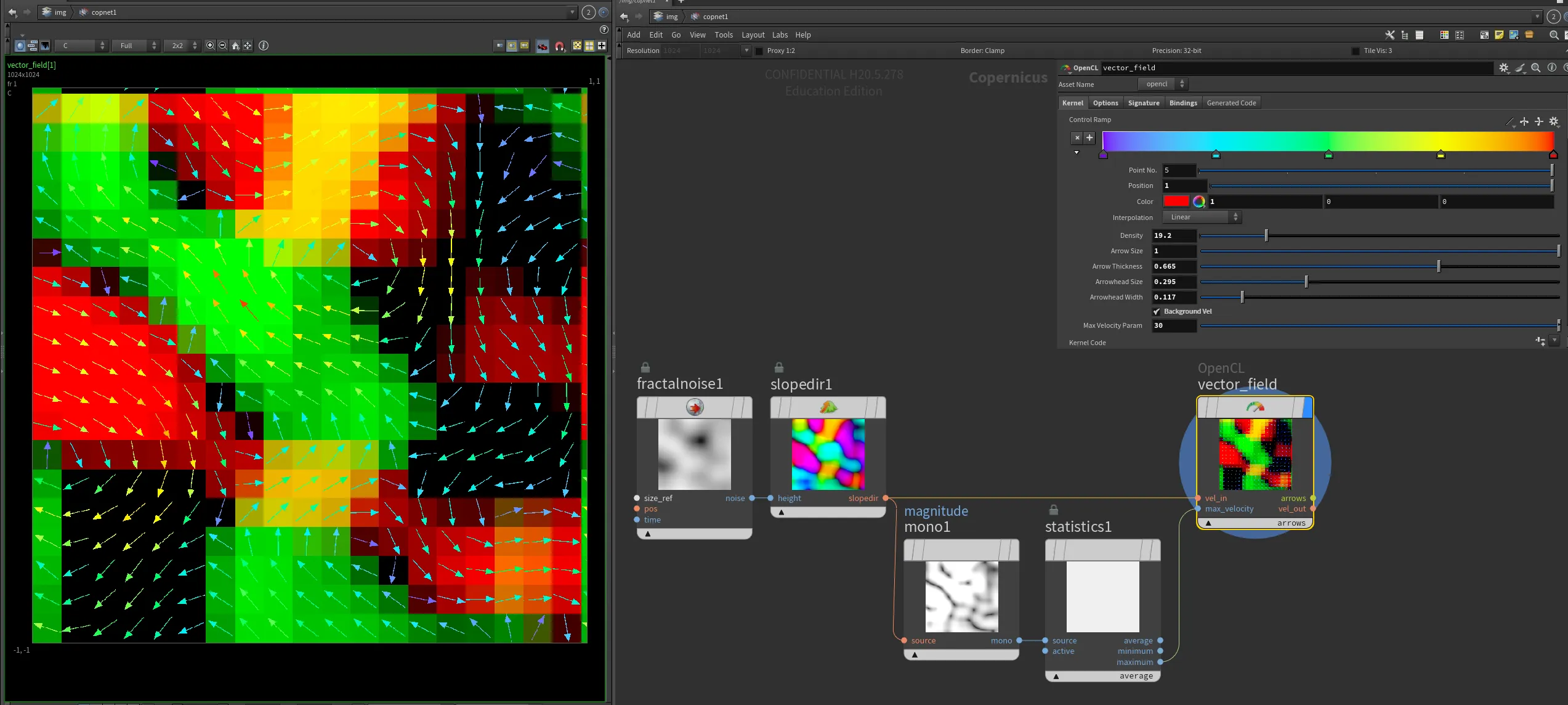
Displaying Vector Fields in COPs
With powerfull COPs, where we can create a 2d solver, it would be great to have the ability to display vector fields directly in COP network. Therefore, I have created an OpenCL node that draws arrows to visualize an input 2D vector (float2) field.
Here's the OpenCL code for the node:
#bind layer vel_in? float2
#bind layer max_velocity? float
#bind layer !&vel_out float2
#bind layer !&arrows float4
#bind ramp control_ramp float3 val=0
#bind parm density float val=1
#bind parm arrow_size float val=1
#bind parm arrow_thickness float val=2
#bind parm arrowhead_size float val=0.1
#bind parm arrowhead_width float val=0.05
#bind parm max_velocity_param float val=10.0
#bind parm background_vel int val=1

bool pointInTriangle(float2 pt, float2 v1, float2 v2, float2 v3)
{
    float2 d1 = v2 - v1;
    float2 d2 = v3 - v2;
    float2 d3 = v1 - v3;

    float2 p1 = pt - v1;
    float2 p2 = pt - v2;
    float2 p3 = pt - v3;

    float cross1 = d1.x * p1.y - d1.y * p1.x;
    float cross2 = d2.x * p2.y - d2.y * p2.x;
    float cross3 = d3.x * p3.y - d3.y * p3.x;

    return (cross1 >= 0 && cross2 >= 0 && cross3 >= 0) || (cross1 <= 0 && cross2 <= 0 && cross3 <= 0);
}

@KERNEL
{
    float2 region = convert_float2(@res) / @density;
    float2 fxy = convert_float2(@ixy);

    // Determine the section index
    int2 section_index = convert_int2(floor(fxy / region));

    // Compute the center of the section
    float2 section_center = convert_float2(section_index) * region + region / 2.0f;

    // Sample the velocity at the center of the section
    float2 velocity = @vel_in.bufferSample(section_center);

    // Pass through the velocity to the output layer
    @vel_out.set(@vel_in.bufferSample(fxy));

    // Compute the direction and magnitude of the velocity
    float magnitude = length(velocity);
    float angle = atan2(velocity.y, velocity.x);

    // Attempt to retrieve the maximum velocity from the max_velocity layer, fallback to max_velocity_param if unsuccessful
    float max_velocity = @max_velocity_param;
    if (@max_velocity.bound)
    {
        max_velocity = @max_velocity.bufferSample(convert_float2(0));
    }

    // Calculate the maximum arrow length to fit within the section, ensuring both the stem and arrowhead fit
    float max_arrow_length = @arrow_size * min(region.x, region.y);

    // Calculate the start and end points of the arrow
    float2 arrow_start = section_center - (float2)(cos(angle), sin(angle)) * 0.5f * max_arrow_length;
    float2 arrow_end = section_center + (float2)(cos(angle), sin(angle)) * 0.5f * max_arrow_length;

    // Calculate arrowhead points
    float2 arrow_dir = normalize(arrow_end - arrow_start);
    float2 arrow_perp = (float2)(-arrow_dir.y, arrow_dir.x); // Perpendicular to arrow direction
    float2 arrowhead_left = arrow_end - arrow_dir * @arrowhead_size * max_arrow_length + arrow_perp * @arrowhead_width * max_arrow_length;
    float2 arrowhead_right = arrow_end - arrow_dir * @arrowhead_size * max_arrow_length - arrow_perp * @arrowhead_width * max_arrow_length;

    // Normalize magnitude using the computed maximum velocity
    float normalized_magnitude = clamp(magnitude / max_velocity, 0.0f, 1.0f);

    // Set the color based on the normalized velocity magnitude using the ramp
    float4 color = (float4)(@control_ramp(normalized_magnitude), 1.0f);

    // Determine if the current pixel is part of the arrow shaft
    float2 dir = normalize(arrow_end - arrow_start);
    float2 to_pixel = fxy - arrow_start;
    float projection_length = dot(to_pixel, dir);
    float2 projection = dir * projection_length;
    float2 arrow_to_pixel = to_pixel - projection;

    bool on_arrow_shaft = projection_length >= 0.0f && projection_length <= length(arrow_end - arrow_start) && length(arrow_to_pixel) <= @arrow_thickness;

    // Determine if the current pixel is part of the arrowhead
    bool on_arrowhead = pointInTriangle(fxy, arrow_end, arrowhead_left, arrowhead_right);

    // Initialize to zero to ensure no stray values
    @arrows.set(0);

    if (on_arrow_shaft || on_arrowhead)
    {
        @arrows.set(color);
    }
    else if (@background_vel == 1)
    {
        @arrows.set((float4)(velocity, 0.0f, 1.0f)); // Pass through the velocity as background
    }
}
This OpenCL kernel visualizes a 2D vector field by drawing arrows to represent the direction and magnitude of the vectors. The code uses various parameters to control the appearance and behavior of the arrows, such as their size, thickness, and color.
By incorporating this OpenCL node into your COPs workflow, you can effectively visualize vector fields, providing a powerful tool for analyzing and understanding complex 2D data.
This is of course not the only way of achieving this effect. An alternative could be stamping arrow shapes onto points in the Copernicus network.
Procedural Caustics
Procedural Caustics!
Procedural caustics is an ongoing topic within the CG community. There have been many more and less sucessfull aproaches. Recently I stubled upon an interesting idea posted by Oneleven on the shadertoy site: 'Sample vector map in the neighborhood of each pixel, then pretend that you move these neighboring pixels according to vector map, then calculate how many of them lands in the current pixel, then normalize that value'.
To verify same result, I have also re-implemented simplex noise and his hacky derivative calculation. Results are amazing and fast and seamless!
We can use other noise types as well!
Current implementation is using sampleBuffer (as I was matching to the reference), therefore it will be resolution dependent, but swapping it into a imageBuffer or textureBuffer should be very simple and resolution independent.
For better explanation, you can also check out sop caustics implementation