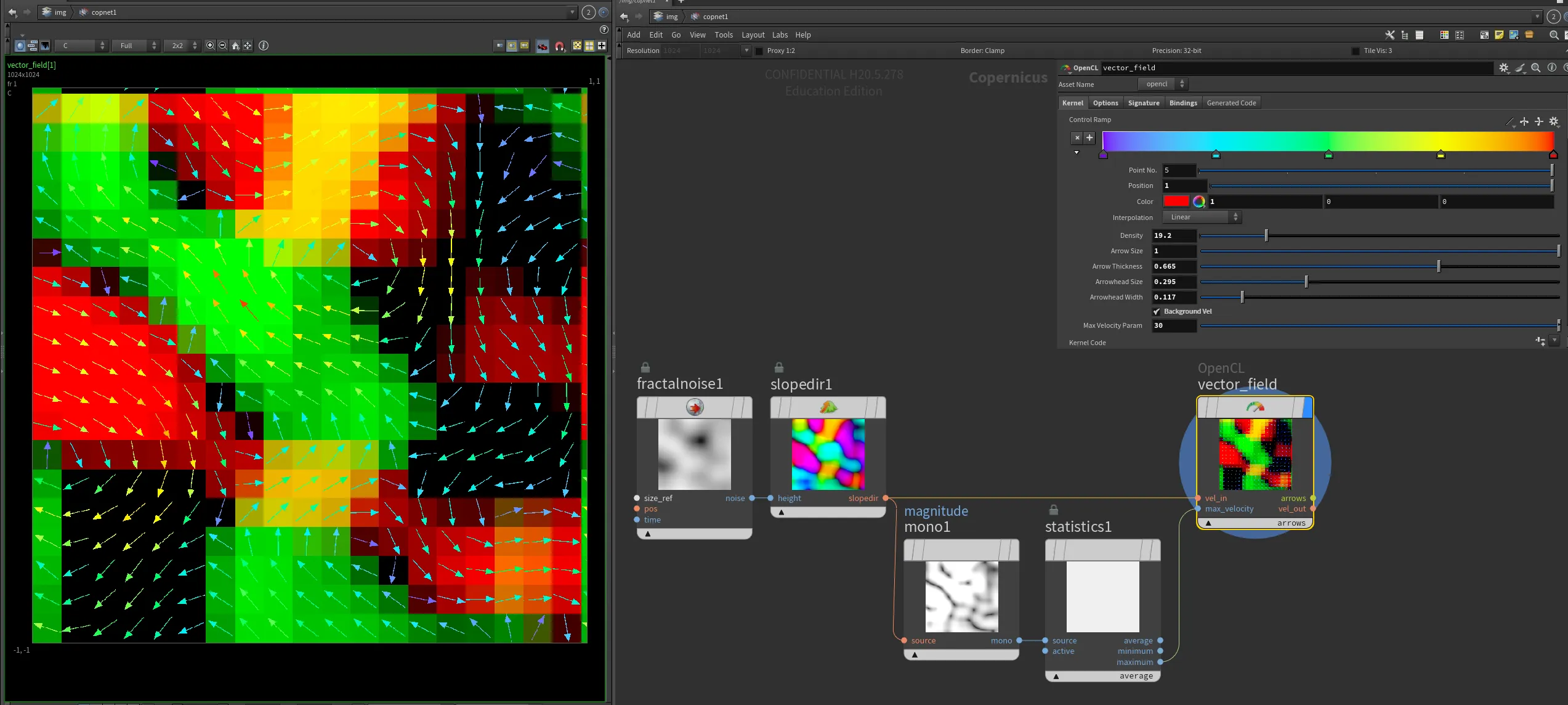
Displaying Vector Fields in COPs

#bind layer vel_in? float2
#bind layer max_velocity? float
#bind layer !&vel_out float2
#bind layer !&arrows float4
#bind ramp control_ramp float3 val=0
#bind parm density float val=1
#bind parm arrow_size float val=1
#bind parm arrow_thickness float val=2
#bind parm arrowhead_size float val=0.1
#bind parm arrowhead_width float val=0.05
#bind parm max_velocity_param float val=10.0
#bind parm background_vel int val=1

bool pointInTriangle(float2 pt, float2 v1, float2 v2, float2 v3)
{
    float2 d1 = v2 - v1;
    float2 d2 = v3 - v2;
    float2 d3 = v1 - v3;

    float2 p1 = pt - v1;
    float2 p2 = pt - v2;
    float2 p3 = pt - v3;

    float cross1 = d1.x * p1.y - d1.y * p1.x;
    float cross2 = d2.x * p2.y - d2.y * p2.x;
    float cross3 = d3.x * p3.y - d3.y * p3.x;

    return (cross1 >= 0 && cross2 >= 0 && cross3 >= 0) || (cross1 <= 0 && cross2 <= 0 && cross3 <= 0);
}

@KERNEL
{
    float2 region = convert_float2(@res) / @density;
    float2 fxy = convert_float2(@ixy);

    // Determine the section index
    int2 section_index = convert_int2(floor(fxy / region));

    // Compute the center of the section
    float2 section_center = convert_float2(section_index) * region + region / 2.0f;

    // Sample the velocity at the center of the section
    float2 velocity = @vel_in.bufferSample(section_center);

    // Pass through the velocity to the output layer
    @vel_out.set(@vel_in.bufferSample(fxy));

    // Compute the direction and magnitude of the velocity
    float magnitude = length(velocity);
    float angle = atan2(velocity.y, velocity.x);

    // Attempt to retrieve the maximum velocity from the max_velocity layer, fallback to max_velocity_param if unsuccessful
    float max_velocity = @max_velocity_param;
    if (@max_velocity.bound)
    {
        max_velocity = @max_velocity.bufferSample(convert_float2(0));
    }

    // Calculate the maximum arrow length to fit within the section, ensuring both the stem and arrowhead fit
    float max_arrow_length = @arrow_size * min(region.x, region.y);

    // Calculate the start and end points of the arrow
    float2 arrow_start = section_center - (float2)(cos(angle), sin(angle)) * 0.5f * max_arrow_length;
    float2 arrow_end = section_center + (float2)(cos(angle), sin(angle)) * 0.5f * max_arrow_length;

    // Calculate arrowhead points
    float2 arrow_dir = normalize(arrow_end - arrow_start);
    float2 arrow_perp = (float2)(-arrow_dir.y, arrow_dir.x); // Perpendicular to arrow direction
    float2 arrowhead_left = arrow_end - arrow_dir * @arrowhead_size * max_arrow_length + arrow_perp * @arrowhead_width * max_arrow_length;
    float2 arrowhead_right = arrow_end - arrow_dir * @arrowhead_size * max_arrow_length - arrow_perp * @arrowhead_width * max_arrow_length;

    // Normalize magnitude using the computed maximum velocity
    float normalized_magnitude = clamp(magnitude / max_velocity, 0.0f, 1.0f);

    // Set the color based on the normalized velocity magnitude using the ramp
    float4 color = (float4)(@control_ramp(normalized_magnitude), 1.0f);

    // Determine if the current pixel is part of the arrow shaft
    float2 dir = normalize(arrow_end - arrow_start);
    float2 to_pixel = fxy - arrow_start;
    float projection_length = dot(to_pixel, dir);
    float2 projection = dir * projection_length;
    float2 arrow_to_pixel = to_pixel - projection;

    bool on_arrow_shaft = projection_length >= 0.0f && projection_length <= length(arrow_end - arrow_start) && length(arrow_to_pixel) <= @arrow_thickness;

    // Determine if the current pixel is part of the arrowhead
    bool on_arrowhead = pointInTriangle(fxy, arrow_end, arrowhead_left, arrowhead_right);

    // Initialize to zero to ensure no stray values
    @arrows.set(0);

    if (on_arrow_shaft || on_arrowhead)
    {
        @arrows.set(color);
    }
    else if (@background_vel == 1)
    {
        @arrows.set((float4)(velocity, 0.0f, 1.0f)); // Pass through the velocity as background
    }
}